Mathematical Preprint Trend Analysis
I analyzed the trend of Mathematical Preprint for the last 15 years.
We’ll begin by gathering data spanning from 2009 to 2023 via the arXiv’s OAI API. Our objective is to explore and identify any significant trends within this dataset.
import pandas as pd
import matplotlib.pyplot as plt
import requests
import pickle
import xml.etree.ElementTree as ET
import time
import numpy as np

for i in range(2009, 2024):
    # Specify the base URL of the OAI-PMH interface
    base_url = 'http://export.arxiv.org/oai2'

    # Specify the verb
    verb = 'ListRecords'

    # Specify the metadata format
    metadata_prefix = 'oai_dc'

    # Formulate the URL
    url = f'http://export.arxiv.org/oai2?verb=ListRecords&set=math&metadataPrefix=oai_dc&from={i}-01-01&until={i}-12-31'

    # An empty list to hold all the XML responses
    responses = []

    while url is not None:
        # Send the GET request
        response = requests.get(url)

        # If the request was successful, parse the data
        if response.status_code == 200:
            responses.append(response.text)
            root = ET.fromstring(response.text)
            token_element = root.find('.//{http://www.openarchives.org/OAI/2.0/}resumptionToken')
            if token_element is not None:
                token = token_element.text
                # Form the new url using the resumption token
                url = f'{base_url}?verb={verb}&resumptionToken={token}'
                print(token)
            else:
                url = None  # No more pages
        else:
            print(f'Request failed with status code {response.status_code}')
            url = None  # Exit the loop
        time.sleep(5)
    with open(f'math_{i}.pkl','wb') as f:
        pickle.dump(responses, f)
# Initialize an empty list and load the list for all years
arXiv_data=[]
for i in range(2009, 2024):
    # Load the list from the file
    with open(f'math_{i}.pkl', 'rb') as f:
        arXiv_data.append(pickle.load(f))
# namespace is used to avoid name conflicts.
namespaces = {'default':'http://www.openarchives.org/OAI/2.0/',
              'oai_dc':'http://www.openarchives.org/OAI/2.0/oai_dc/',
              'dc':'http://purl.org/dc/elements/1.1/'}
def get_titles(list):
    titles = []
    for i in range(len(list)):
        root = ET.fromstring(list[i])
        for record in root.findall('default:ListRecords/default:record', namespaces):
            title = record.findall('default:metadata/oai_dc:dc/dc:title', namespaces)
            if len(title)>0:
                titles.append(title[0].text)
            else: titles.append(None)
    return titles
def get_descriptions(list):
    descriptions = []
    for i in range(len(list)):
        root = ET.fromstring(list[i])
        for record in root.findall('default:ListRecords/default:record', namespaces):
            description = record.findall('default:metadata/oai_dc:dc/dc:description', namespaces)
            if len(description)>0:
                descriptions.append(description[0].text)
            else: descriptions.append(None)
    return descriptions
def get_areas(list, subject):
    area_list = []
    for i in range(len(list)):
        root = ET.fromstring(list[i])
        for record in root.findall('default:ListRecords/default:record', namespaces):
            areas = record.findall('default:metadata/oai_dc:dc/dc:subject', namespaces)
            areas_for_this_subject = [area.text for area in areas
                                            if subject in area.text]
            area_list.append(areas_for_this_subject)
    return area_list
def get_authors(list):
    authors = []
    for i in range(len(list)):
        root = ET.fromstring(list[i])
        for creator in root.findall('default:ListRecords/default:record', namespaces):
            author_set = creator.findall('default:metadata/oai_dc:dc/dc:creator', namespaces)
            authors.append([author.text for author in author_set])
    return authors
#separate this given its unique characteristics
def get_dates(list):
    dates = []
    for i in range(len(list)):
        root = ET.fromstring(list[i])
        for record in root.findall('default:ListRecords/default:record', namespaces):
            date = record.findall('default:header/default:datestamp', namespaces)
            dates.append(date[0].text)
    return dates
# This function will create our desired DataFrame
def DataFrame_from_responses(list, subject):
    return pd.DataFrame({'authors':get_authors(list),
    'title':get_titles(list),
    'date':get_dates(list),
    'description':get_descriptions(list),
    'area':get_areas(list, subject)})
# Initialize an empty dictionary to hold the dataframes
df_dict = {}

# Loop over the years
for year in range(2009, 2024):
    # Create a dataframe and store it in the dictionary
    df_dict[year] = DataFrame_from_responses(arXiv_data[year-2009], 'Math')
years = []
lengths = []

for year, df in df_dict.items():
    years.append(year)
    lengths.append(df.shape[0])

plt.figure(figsize=(10,6))
plt.plot(years, lengths, marker='o', linestyle='-', color='b')
plt.plot(years, lengths)
plt.title('Number of preprints by year')
plt.xlabel('Year')
plt.ylabel('Number of preprint')
plt.annotate('Ongoing Data', (years[-1], lengths[-1]), textcoords="offset points", xytext=(-10,-15), ha='center', fontsize=12, color='r')
plt.grid()
plt.tight_layout()
plt.xticks(np.arange(min(years), max(years) + 1, 1))
plt.show()

The volume of the preprints in math is increasing every year. Let us compute the yearly average count of authors for each preprint by year.
years=[]
avg_num_authors=[]

for year, df in df_dict.items():
    years.append(year)
    num_authors=df['authors'].apply(len)
    avg_num_authors.append(num_authors.mean())

plt.figure(figsize=(10,6))
plt.plot(years, avg_num_authors, marker='o', linestyle='-', color='b')
plt.plot(years, avg_num_authors)
plt.title('Average number of authors for each preprint by year')
plt.xlabel('Year')
plt.ylabel('Average number of authors')
plt.annotate('Ongoing Data', (years[-1], avg_num_authors[-1]), textcoords="offset points", xytext=(-10,-15), ha='center', fontsize=12, color='r')
plt.grid()
plt.tight_layout()
plt.xticks(np.arange(min(years), max(years) + 1, 1))
plt.show()
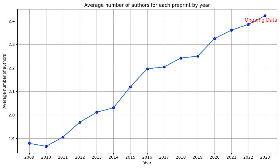
The increasing trend of collaboration in mathematics could account for the surge in preprint production, as seen in the prior chart.
area_counts_by_year = []
for i in range(2009, 2024):
    # Explode the 'area' column
    exploded_df = df_dict[i].explode('area')

    # Count the frequency of each area
    area_counts = exploded_df['area'].value_counts()

    # This will count the number of subject areas in data
    for i in range(len(area_counts)):
        if "Mathematics" in area_counts.index[i]:
            area_counts.index = area_counts.index.str.replace("Mathematics - ", "")

    # create a boolean mask where True for rows whose index does not start with a number
    mask = ~area_counts.index.str[0].str.isdigit()

    # apply the mask to the DataFrame. This will delete the ones with MSC classification code
    area_counts_by_year.append(area_counts[mask])
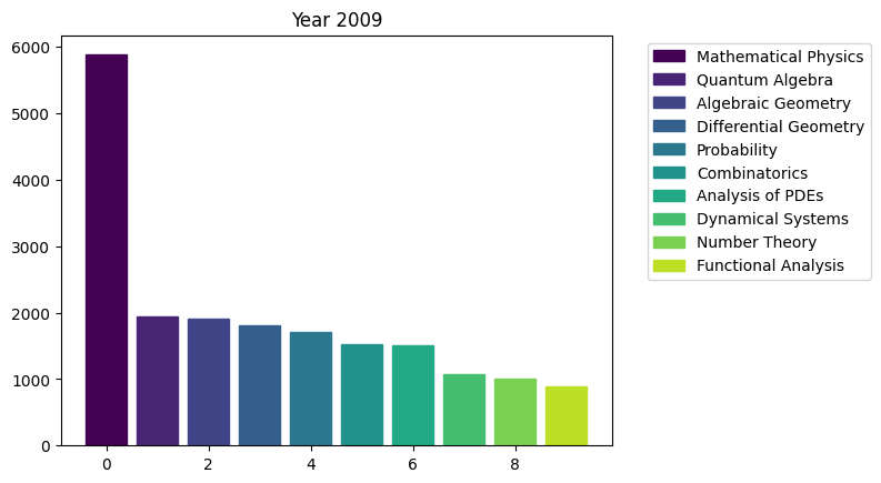
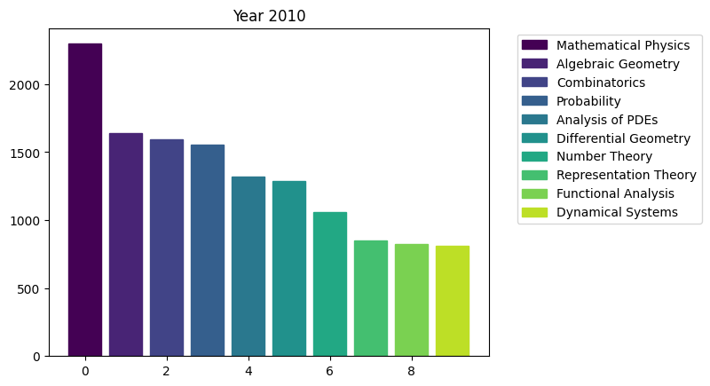
# Let us plot the number of areas of research for each year
for i in range(15):
    fig, ax = plt.subplots()

    bars = ax.bar(range(10), area_counts_by_year[i].values[:10])  # plot bars

    for j in range(10):
        bars[j].set_color(plt.cm.viridis(j / 10.))  # set a different color for each bar
    plt.title(f'Year {i+2009}')
    ax.legend(bars, area_counts_by_year[i].index[:10], bbox_to_anchor=(1.05, 1), loc='upper left')  # add a legend outside of the plot
    plt.show()
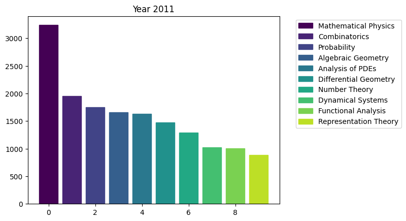
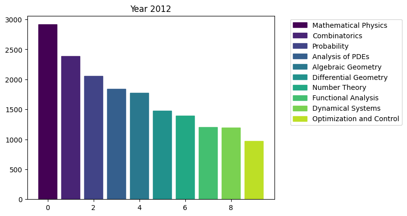
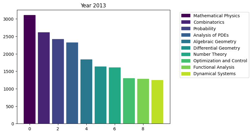
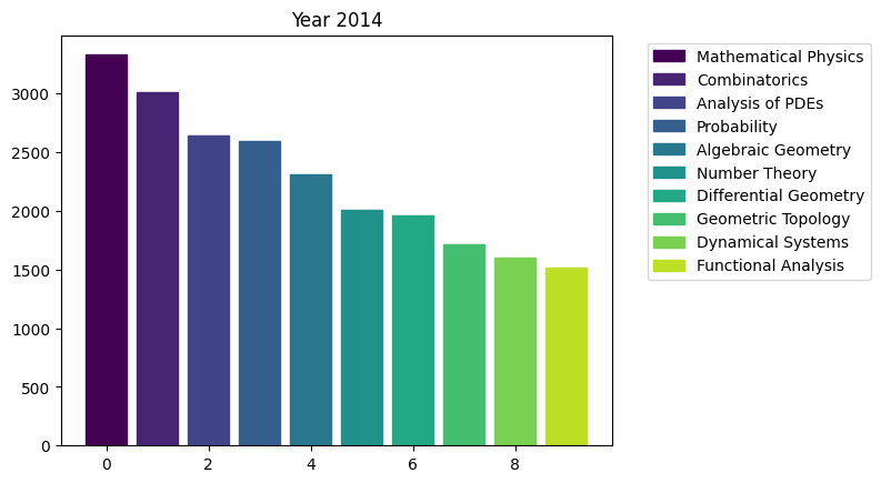
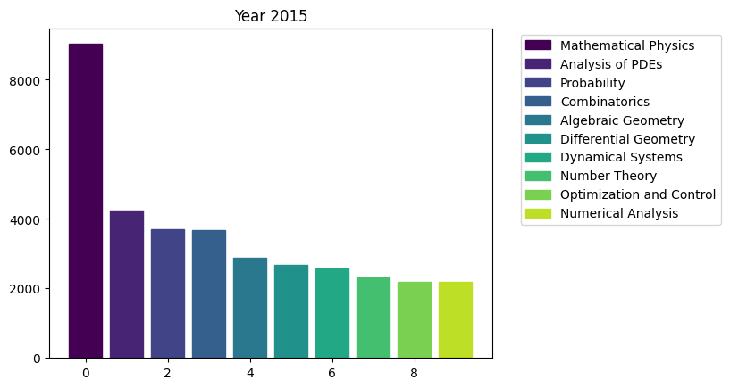
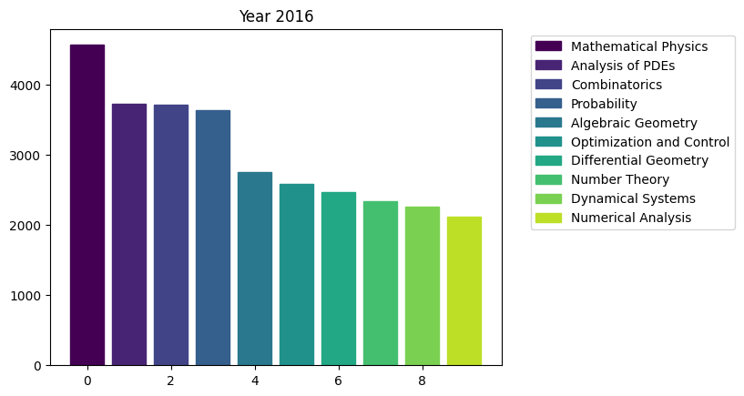
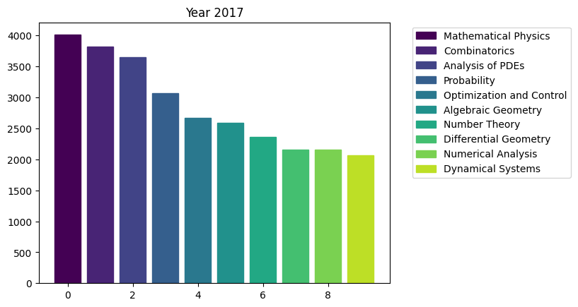
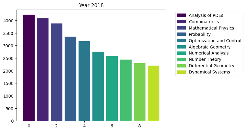
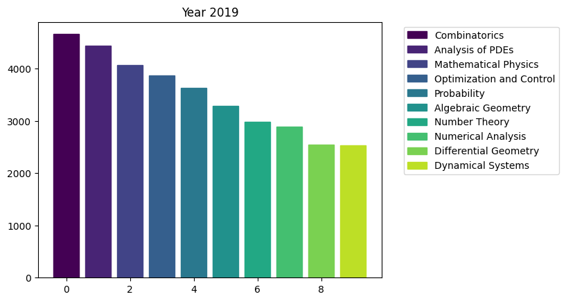
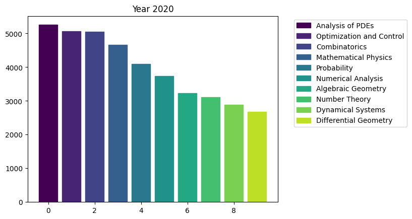
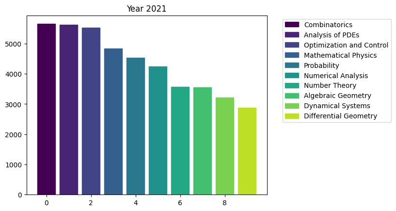
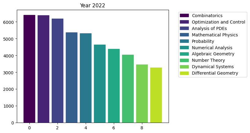
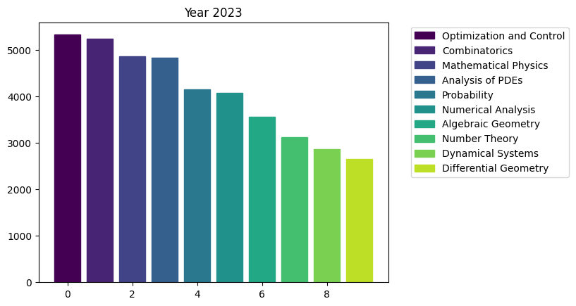
We can see the rapid surge of Optimization and Control community.
years = range(2009, 2024)
OC = [area_counts_by_year[i]['Optimization and Control'] for i in range(15)]
plt.figure(figsize=(10,6))
plt.plot(years, OC, marker='o', linestyle='-', color='b')
plt.plot(years, OC)
plt.title('Number of preprints for Optimization and Control by year')
plt.xlabel('Year')
plt.ylabel('Optimization and Control')
plt.annotate('Ongoing Data', (years[-1], OC[-1]), textcoords="offset points", xytext=(-10,-15), ha='center', fontsize=12, color='r')
plt.grid()
plt.tight_layout()
plt.xticks(np.arange(min(years), max(years) + 1, 1))
plt.show()
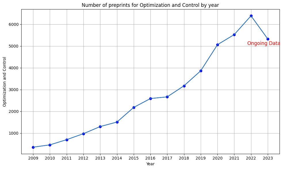
We can also compare the average slope, for example between Optimization/Control and Algebraic Geometry.
OC = (area_counts_by_year[13]['Optimization and Control']
      -area_counts_by_year[0]['Optimization and Control'])/14

AG = (area_counts_by_year[13]['Algebraic Geometry']
      -area_counts_by_year[0]['Algebraic Geometry'])/14

print(f'Average increasing rate of Optimization community is {round(OC, 2)} and that of Algebraic Geometry community is {round(AG, 2)}.')
Average increasing rate of Optimization community is 430.79 and that of Algebraic Geometry community is 177.14.
import re
import string

def clean_and_split(s):
    #'tr' is an object that will assign blank space to each
    # punctuation symbol
    tr=str.maketrans(string.punctuation," "*len(string.punctuation))
    s=s.lower().translate(tr)
    # \r\n and \n are line breaks; we substitute with blank space.
    s=re.sub('(\r\n)+',' ',s)
    s=re.sub('(\n)+',' ',s)
    # replace all multiple spaces into a single space.
    s=re.sub(' +',' ',s.strip())
    s=s.split(' ')
    return s
# For all descriptions, we split all words and count them.
list_of_words = df_dict[2009]['description'].dropna().apply(clean_and_split)
list_of_words_flattened = [a for b in list_of_words for a in b]
word_counts_1=collections.Counter(list_of_words_flattened)

# We are interested in the change of keywords in 15 years so we collect words for year 2023 as well
list_of_words = df_dict[2023]['description'].dropna().apply(clean_and_split)
list_of_words_flattened = [a for b in list_of_words for a in b]
word_counts_2=collections.Counter(list_of_words_flattened)
nltk.download('brown')
nltk.download('words')
# Calculate frequencies of each word in the Brown corpus
fdist_brown = nltk.FreqDist(w.lower() for w in brown.words())
# Create a set of English words
english_words = set(words.words())
# Extract only the words that are in the dictionary
# and used 1000 times more frequently in my data than in the Brown corpus.
unusually_frequent_words_1 = {word: count for word, count in word_counts_1.items()
if word in english_words and count > 1000 * fdist_brown[word]}
unusually_frequent_words_2 = {word: count for word, count in word_counts_2.items()
if word in english_words and count > 1000 * fdist_brown[word]}
# Create a WordCloud object
wordcloud_1 = WordCloud(width=800, height=400, background_color='white').generate_from_frequencies(unusually_frequent_words_1)
wordcloud_2 = WordCloud(width=800, height=400, background_color='white').generate_from_frequencies(unusually_frequent_words_2)
# Plot the word cloud
def wordcloud(data, year):
plt.figure(figsize=(10, 5))
plt.imshow(data, interpolation='bilinear')
plt.title(f'Literature keywords for {year} in mathematics', fontsize=20, fontname = 'Arial')
plt.axis('off')
plt.show()
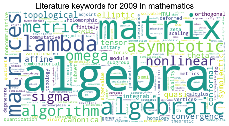
wordcloud(wordcloud_1, 2009)
wordcloud(wordcloud_2, 2023)
[nltk_data] Downloading package brown to
[nltk_data]     /Users/minseoksong/nltk_data...
[nltk_data]   Package brown is already up-to-date!
[nltk_data] Downloading package words to
[nltk_data]     /Users/minseoksong/nltk_data...
[nltk_data]   Package words is already up-to-date!
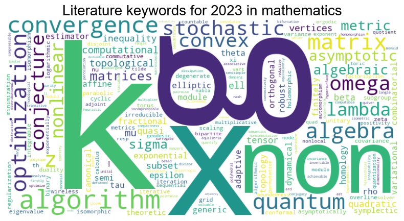
Some words ‘g,’ ‘k,’ and ‘x’ in year 2023, even if less frequently used, are awkward, so we may delete them.
del unusually_frequent_words_2['g']
del unusually_frequent_words_2['k']
del unusually_frequent_words_2['x']
# We display the keywords for 2023 as before.
wordcloud_2 = WordCloud(width=800, height=400, background_color='white').generate_from_frequencies(unusually_frequent_words_2)
wordcloud(wordcloud_2, 2023)
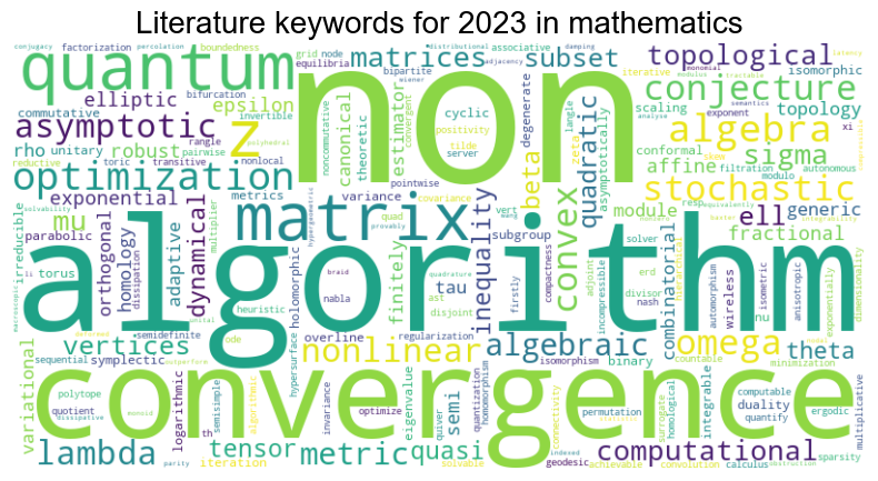
The prominence of ‘algorithm’ as a keyword is likely a reflection of the growing interest and investment in the optimization and control community, as evidenced by previous bar graphs depicting research areas.